Unraveling High-Dimensional Data: A Comprehensive Guide To UMAP And T-SNE

Unraveling High-Dimensional Data: A Comprehensive Guide to UMAP and t-SNE

Related Articles: Unraveling High-Dimensional Data: A Comprehensive Guide to UMAP and t-SNE

Introduction

With enthusiasm, let’s navigate through the intriguing topic related to Unraveling High-Dimensional Data: A Comprehensive Guide to UMAP and t-SNE. Let’s weave interesting information and offer fresh perspectives to the readers.

Unraveling High-Dimensional Data: A Comprehensive Guide to UMAP and t-SNE

In the realm of data analysis, high-dimensional datasets pose a significant challenge. Visualizing and understanding the intricate relationships within such datasets can be a daunting task. This is where dimensionality reduction techniques like Uniform Manifold Approximation and Projection (UMAP) and t-Distributed Stochastic Neighbor Embedding (t-SNE) come into play. These powerful algorithms offer a solution to the dimensionality curse, enabling us to explore and analyze complex data in a more intuitive and manageable manner.

This article aims to provide a comprehensive understanding of UMAP and t-SNE, exploring their underlying principles, strengths, and limitations. By delving into their intricacies, we aim to shed light on their crucial role in data visualization and exploration.

Understanding the Challenge: The Curse of Dimensionality

Imagine a dataset with thousands of features, each representing a different aspect of the data. Visualizing such high-dimensional data becomes an insurmountable task. The human brain is adept at understanding two or three dimensions, but beyond that, our cognitive abilities struggle to grasp the complexities. This phenomenon, known as the curse of dimensionality, hinders our ability to analyze and interpret data effectively.

Dimensionality reduction techniques address this challenge by projecting the high-dimensional data onto a lower-dimensional space, typically two or three dimensions. This projection aims to preserve the essential relationships and structure of the original data while reducing the number of features.

UMAP: A Topological Approach to Dimensionality Reduction

UMAP stands out as a relatively new but highly effective dimensionality reduction technique. It leverages the power of topology, a branch of mathematics concerned with the study of shapes and spaces. UMAP utilizes a topological approach to capture the global structure of the data, ensuring that nearby points in the high-dimensional space remain close in the reduced space.

Key Features of UMAP:

• Topological Data Analysis: UMAP uses topological data analysis to model the underlying manifold of the data. This approach allows it to preserve the global structure of the data, even when dealing with complex, non-linear relationships.
• Local and Global Structure Preservation: UMAP strives to preserve both local and global relationships within the data. This ensures that not only nearby points but also clusters and overall patterns are faithfully represented in the reduced space.
• Scalability: UMAP is designed to handle large datasets efficiently, making it suitable for real-world applications with massive amounts of data.
• Flexibility: UMAP offers a wide range of parameters that can be adjusted to fine-tune the reduction process, allowing users to tailor the algorithm to their specific needs.

How UMAP Works:

1. Constructing a Neighborhood Graph: UMAP begins by constructing a k-nearest neighbor graph, connecting points that are close to each other in the high-dimensional space. This graph represents the local structure of the data.
2. Mapping to a Low-Dimensional Space: UMAP then maps this graph to a lower-dimensional space using a cost function that minimizes the distance between connected points in the graph. This mapping ensures that the local relationships are preserved.
3. Global Structure Preservation: By employing a topological approach, UMAP also preserves the global structure of the data. This ensures that clusters and overall patterns are faithfully represented in the reduced space.

t-SNE: Embracing Probabilistic Relationships

t-SNE, a widely-used dimensionality reduction technique, approaches the problem by focusing on probabilistic relationships between data points. It aims to preserve the relative distances between points in the high-dimensional space by mapping them to a lower-dimensional space.

Key Features of t-SNE:

• Probabilistic Approach: t-SNE uses a probabilistic approach to model the relationships between data points. It assigns a probability to each pair of points, reflecting the likelihood of them being neighbors in the high-dimensional space.
• Local Structure Preservation: t-SNE focuses on preserving the local structure of the data, ensuring that nearby points remain close in the reduced space.
• Non-Linear Mapping: t-SNE allows for non-linear mappings, enabling it to capture complex, non-linear relationships within the data.

How t-SNE Works:

1. Calculating Similarity Probabilities: t-SNE first calculates the probability of two points being neighbors in the high-dimensional space based on their Euclidean distance.
2. Mapping to a Low-Dimensional Space: It then maps these probabilities to a lower-dimensional space, minimizing the Kullback-Leibler divergence between the probability distributions in the high-dimensional and low-dimensional spaces. This ensures that the local relationships are preserved.

UMAP vs. t-SNE: A Comparative Analysis

While both UMAP and t-SNE are powerful dimensionality reduction techniques, they differ in their underlying principles and strengths.

• Global vs. Local Focus: UMAP emphasizes preserving both local and global structure, while t-SNE primarily focuses on preserving local relationships.
• Scalability: UMAP is designed to handle large datasets efficiently, making it more scalable than t-SNE.
• Computational Complexity: t-SNE tends to be more computationally demanding, especially for large datasets.
• Parameter Tuning: UMAP offers more flexibility in parameter tuning, allowing users to tailor the algorithm to their specific needs.

The choice between UMAP and t-SNE depends on the specific requirements of the analysis. If global structure preservation is crucial, UMAP is the preferred choice. However, if computational efficiency is a priority, t-SNE may be a better option for smaller datasets.

Applications of UMAP and t-SNE

UMAP and t-SNE find widespread applications in various fields, including:

• Data Visualization: These techniques are invaluable for visualizing high-dimensional data, allowing us to identify clusters, outliers, and other patterns that might be hidden in the original data.
• Machine Learning: UMAP and t-SNE can be used as preprocessing steps in machine learning algorithms, reducing the dimensionality of the data and improving the performance of models.
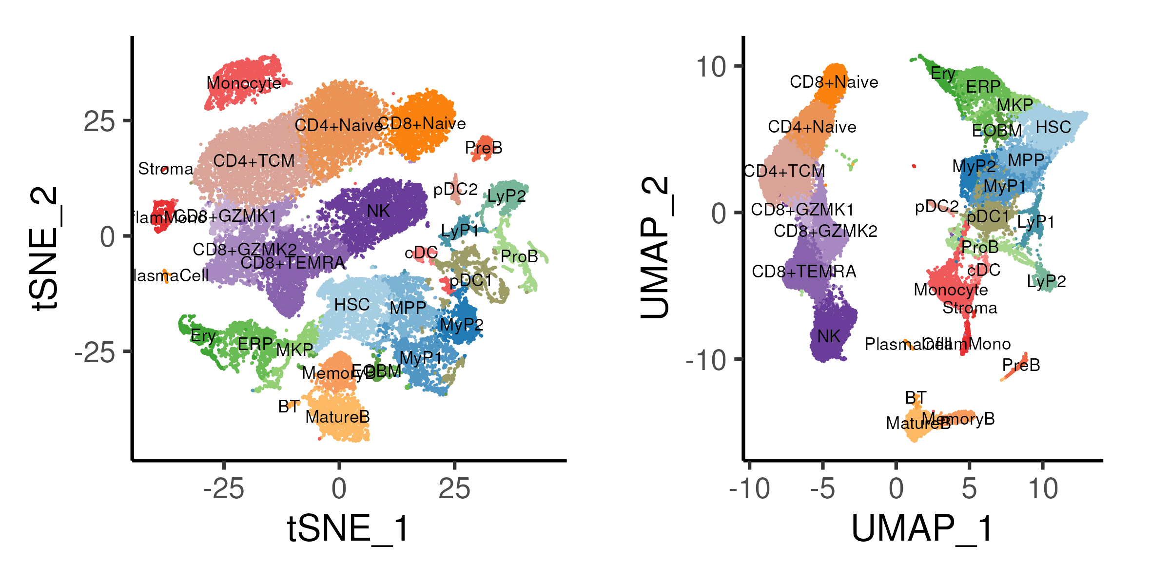
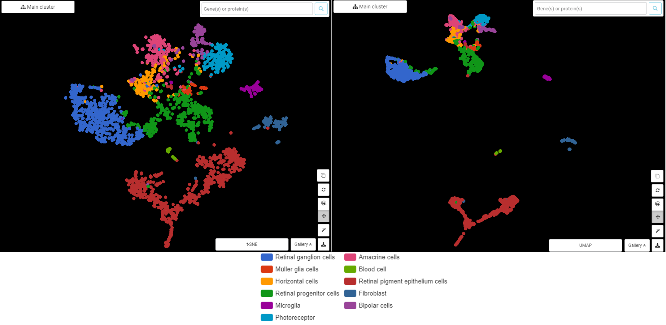
• Bioinformatics: In bioinformatics, UMAP and t-SNE are used to analyze gene expression data, identify different cell types, and explore the relationships between different biological entities.
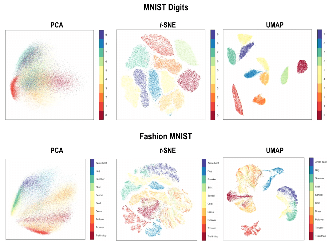
• Image Processing: These techniques can be applied to image data, allowing us to extract meaningful features and perform image classification tasks.

FAQs about UMAP and t-SNE

1. What are the main differences between UMAP and t-SNE?

UMAP emphasizes preserving both local and global structure, while t-SNE primarily focuses on preserving local relationships. UMAP is more scalable and computationally efficient than t-SNE, making it suitable for larger datasets.

2. When should I use UMAP instead of t-SNE?

If global structure preservation is crucial for your analysis, UMAP is the preferred choice. It is also more suitable for large datasets due to its scalability.

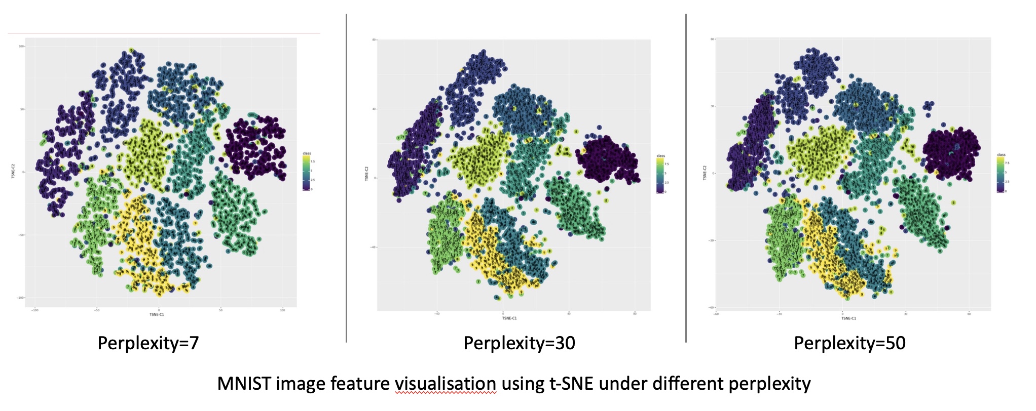
3. How can I choose the optimal parameters for UMAP and t-SNE?

The optimal parameters for UMAP and t-SNE depend on the specific dataset and the desired outcome. Experimenting with different parameter values and visualizing the results is essential to find the best configuration.

4. Can I use UMAP or t-SNE for categorical data?

While UMAP and t-SNE are primarily designed for numerical data, they can also be used for categorical data by encoding the categories into numerical values.

5. Are there any limitations to UMAP and t-SNE?

Both UMAP and t-SNE can struggle with datasets containing high levels of noise or outliers. They can also be sensitive to the choice of parameters, requiring careful tuning to obtain meaningful results.

Tips for Using UMAP and t-SNE

• Data Preprocessing: Before applying UMAP or t-SNE, it is crucial to preprocess the data appropriately. This includes scaling the features, handling missing values, and removing outliers.
• Parameter Tuning: Experiment with different parameter values to find the best configuration for your specific dataset.
• Visualizing Results: Visualize the results of the dimensionality reduction to assess the quality of the projection and identify any potential issues.
• Understanding the Limitations: Be aware of the limitations of UMAP and t-SNE, such as their sensitivity to noise and outliers.
• Combining with Other Techniques: Consider combining UMAP or t-SNE with other techniques, such as clustering or classification, to gain further insights from the data.

Conclusion

UMAP and t-SNE are powerful tools for exploring and analyzing high-dimensional data. They provide a means to visualize complex relationships, identify clusters, and uncover hidden patterns. By leveraging the principles of topology and probability, these techniques offer valuable insights into the structure and organization of data, enabling us to make informed decisions and draw meaningful conclusions.

As the field of data analysis continues to evolve, dimensionality reduction techniques like UMAP and t-SNE will play an increasingly vital role in our ability to understand and interpret the vast and complex datasets that surround us. By understanding their strengths and limitations, we can harness their power to unlock the hidden secrets within data, driving innovation and discovery across various domains.

Closure

Thus, we hope this article has provided valuable insights into Unraveling High-Dimensional Data: A Comprehensive Guide to UMAP and t-SNE. We appreciate your attention to our article. See you in our next article!